ac*ft to MG? k = ⁷¹²⁸⁄₂₁₈₇₅
ac*ft/hr to cfs? k = 121/10
ac*ft to MG? k = ⁷¹²⁸⁄₂₁₈₇₅
ac*ft/hr to cfs? k = 121/10
D=\bigg(\frac{2.16Q\eta}{\sqrt{S}}\bigg)^{3/8}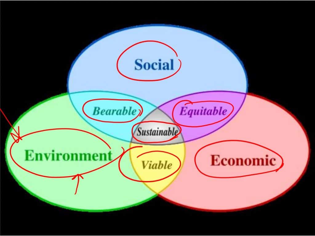
Remember S-E-E, B-E-V
(social, economic, environment — bearable, equitable, viable)
w=\frac{W_w}{W_s}\\ \space \\mc=\frac{W_w}{W_s}Ww = weight of water
Ws = weight of soil solids
weight of soil per unit volume
\gamma=\frac{W_t}{V_t}Wt =
Vt =
\gamma_d=\frac{W_s}{V_t}Vw = volume of water in the voids
Vv = volume of voids
dry unit weight & soil unit weight and moisture content (w) relationsh
\gamma=\frac{W}{V}=\frac{W_s+W_w}{V}=\frac{W_s(1+w)}{V}\gamma_d=\frac{W_s}{V}\begin{aligned} \gamma &=\frac{W_s(1+w)}{V} \\ \space \\ \frac{\gamma}{(1+w)}&=\frac{W_s\xcancel{(1+w)}}{V} \\ \space \\ \frac{\gamma}{(1+w)}&=\frac{W_s}{V} \\ \space \\ \frac{\gamma}{(1+w)}&=\gamma_d
\end{aligned}Ww = weight of water
Ws = weight of soil solids
porosity commonly expressed relationships
n=\frac{e}{1+e}=\frac{\frac{V_v}{V_s}}{1+\frac{V_v}{V_s}}e = void ratio
Vv = volume of voids
Vs = volume of soil solids
weight of soil per unit volume
\rho=\frac{M}{V}Wt =
Vt =
\rho_d=\frac{M_s}{V_t}ρ = dry density of soil (lb/ft3, slug/ft3)
Ms= mass of soil solids in sample (lb, slug)
V = volume of soil sample (ft3, gal)
= 62.43 lb/ft3
= 8.35 lb/gal
= .0361 lb/in3
= 1.94 slug/ft3
= .259 slug/gal
= .00112 slug/in3
The tip for figuring out problems in this conceptual way, is to make V(soil solids) = 1; and if Vs = 1, Vv = e
W_s=G_s\gamma_w
Gs = specific gravity
ɣw = unit weight of water, (62.43 lb/ft3)
\begin{aligned} W_w&=wG_s\gamma_w \\ &=wW_s\end{aligned}Gs = specific gravity
ɣw = unit weight of water, (62.43 lb/ft3)
Ws = weight of soil solids
specific gravity of solid soils
G_s=\frac{W_s}{V_s\gamma_w}
ɣw = unit weight of water, (62.43 lb/ft3)
V_v=V_w=V_a=e
V_s=1
V_t=1+e
V…
if the soil sample is saturated – that is, the void spaces are completely filled with water – the relationship for saturation unit weight (gamma sat) can be derived in a similar manner:
\gamma_{sat}=\frac{W_t}{V_t}=\frac{W_s+W_w}{V}=\frac{G_s\gamma_w+e\gamma_w}{1+e}=\frac{\gamma_w(G_s+e)}{1+e}Vw = volume of water in the voids
Vv = volume of voids
\begin{aligned} \text{\textdegree}\text{S}&=\frac{V_w}{V_v} \\ \space \\ \text{\textdegree}\text{S}&=\frac{wG_s}{e} \\ \space \\ \text{\textdegree}\text{S}e&=wG_s
\end{aligned}
and with °S = 1… (fully saturated)
e=wG_s
void ratio commonly expressed relationships
\gamma=\frac{W}{V}=\frac{W_s+W_w}{V}=\frac{G_s\gamma_w+wG_s\gamma_w}{1+e}=\frac{(1+w)G_s\gamma_w}{1+e}Vv = volume of voids
Vs = volume of soil solids
\begin{aligned}\gamma_d&=\frac{W_s}{V} \\ \space \\\gamma_d&=\frac{G_s\gamma_w}{1+e} \end{aligned}e = void ratio
Vv = volume of voids
Vs = volume of soil solids
void ratio commonly expressed relationships
\begin{aligned} e &=\frac{G_s\gamma_w}{\gamma_d} -1 \\ \space \\e &= \frac{G_s\gamma_w (1+w)}{\gamma}-1\end{aligned}Vv = volume of voids
Vs = volume of soil solids
\begin{aligned}\gamma_d&=\frac{W_s}{V} \\ \space \\\gamma_d&=\frac{G_s\gamma_w}{1+e} \end{aligned}e = void ratio
Vv = volume of voids
Vs = volume of soil solids
– NFL (National Football League)
– CFL (Canadian Football League)
– LFA (Liga de Fútbol Americano Profesional)
– ELF (European League of Football)
– X-League (Japan)
– USFL (United States Football League)
– PRAFL (Puerto Rico American Football League)
– AFL (Arena Football League)
– AAL (American Arena League)
– IFL (Indoor Football League)
– NAL (National Arena League)
– TAL (The Arena League)
– AFFL (American Flag Football League)
– WFA (Women’s Football Alliance)
– USWFL (United States Women’s Football League)
– Extreme Football League (X-League)
– (MLFL) Liga Mexicana de Football Lingerie
– PGFL (Pretty Girls Football League)
– ILBF (Liga Iberoamericana de Bikini Football)
– NCAA (USA)
– U Sports (Canada)
– HSFA (High School Football Association)
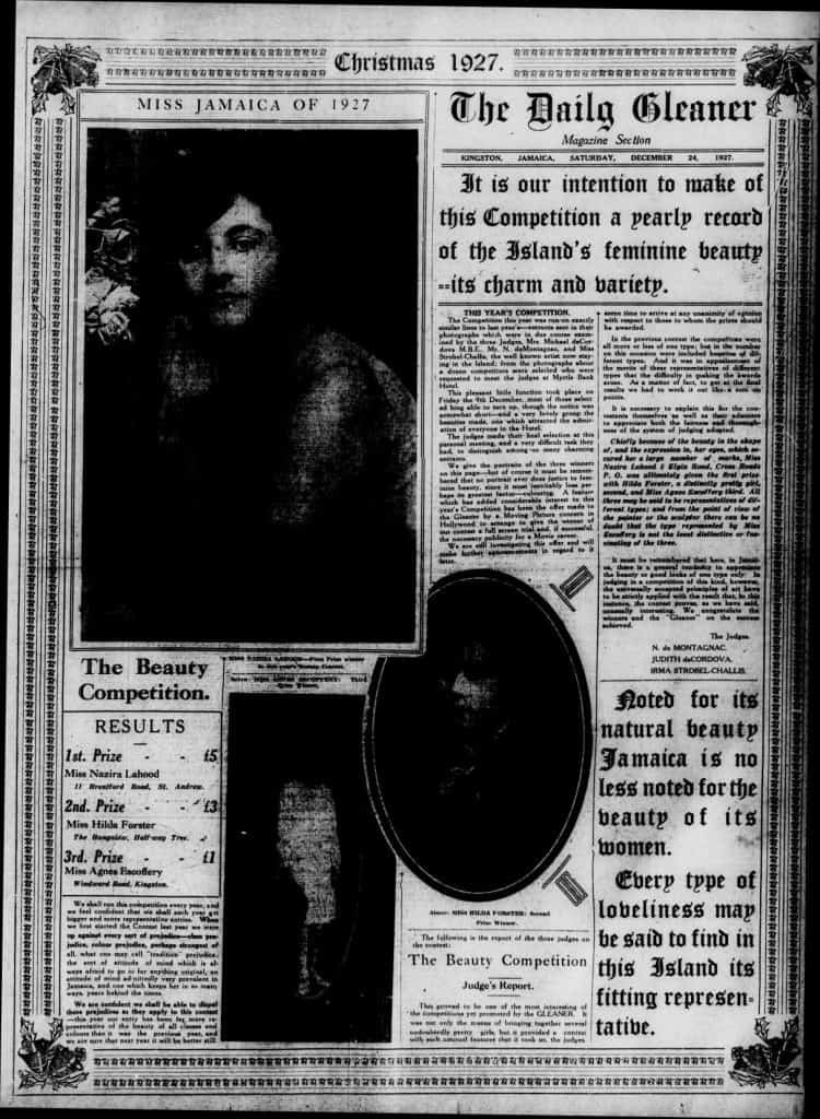
Miss Nazira Lahood won 1st place prize in the ’27 Miss Jamaica Pageant. Her prize was 5 Jamaican pounds (£5). Runners’ up were Miss Hilda Forester from Halfway-Tree in 2nd and Miss Agnes Escofferey from Kingston.
Before I start these posts, I always notify to you (the reader) that while I did take and pass my required 63-hr pre-licensing course for the state of Florida; I, however did not continue pursuing real estate as a career. I am merely a fantastic on the intricacies of real estate.
Stay prepared and stay skilled — Chris, from ChristoAnd.com
Ownership is a right. It is (after all) protected by the law of Federal Government. A title in it of itself means ownership. Ownership of what? of something; literally anything. But usually in terms of property. When a party or person owners property, they have a legal title to said property.
An equitable title is the right to gain ownership interest in the future. This effectively bestows a financial or equitable interest in a property. An estate — which refers to a party that is representive the value that an individual owns (they are usually dead), this is an example of a body that would own such titles. There are multiple types of estates. But we’ll cover that here.
How can a party prove that they are entitled to own something? By acquiring a notice. Without this type of document before obtaining a property, an opposing claimant could contend for ownership. Two types — actual notice, or constructive notice, are used to provide evidence of ownership.
Although constructive and actual have the same call for legal action — using a constructive notice is the best for legal evidence because it records an instrument in the public records which can be easier to prove.
Clear, marketable, or merchantable title to real property is title in fee simple (fee simple is another word for saying the landowner’s total and complete ownership of a land and all the properties that are on it.)
Land ownership in fee simple is free from litigation and defects. To conclude whether or not a title is good and vendible, a record of ownership must be tracked back for a necessary period of time. This is to assure that there is no unresolved or outstanding claims that exist against the title. The time period of such title assessment is called the root of title.
Root of title, in Florida extends back 30 years from the recording of the claim. Claims exceeding 30 years old are extinguished. [F.S. 712] Property rights may be traced back to a land grant from the state or federal government; or from a land grant given by the King of Spain. (Starting in 1790, Spain offered land grants to encourage settlement in the colony of Florida — in 1821, Florida was officially transferred from Spanish to American control)
A chain of title is created when searching for all public records to a piece of real-estate, resulting in a timeline of recorded documents that links all past owners of the land from the roots of the title to the present date. Abstracting and title insurance companies compile these pubic records into a title plant.
Title defects are any claims or other factors that could cause a title to be declared invalid. This could lead a current title to be called into questioning. To combat this, buyers will usually obtain title insurance. This insurance provides a financial protection against losses endured from a defective title. There is no Florida law that requires a borrower to obtain title insurance.
The Kendal, Manchester Railway Disaster of 1957, is one of the most tragic events that has happened in the history of Jamaica. The crash was personally accounted for by my grandfather. He was an engineer that lived in Mandeville, which is under 3 miles away from Kendal. He was on onlooker at the crash site right on the day of the crash — September 1, 1957.
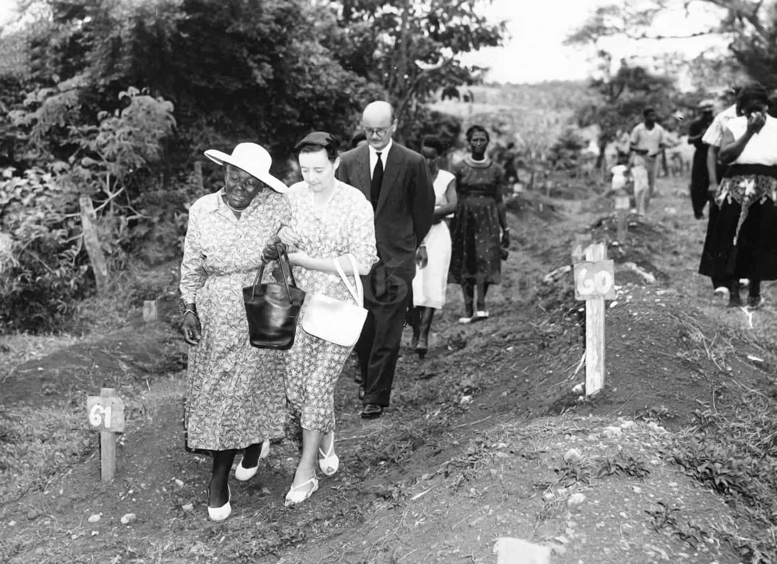
Colonel R. G. Jackson, general manager of the Jamaica Government Railway along with Mrs. Jackson and mourners attending memorial service for the unidentified Kendal train crash victims on Sept. 10
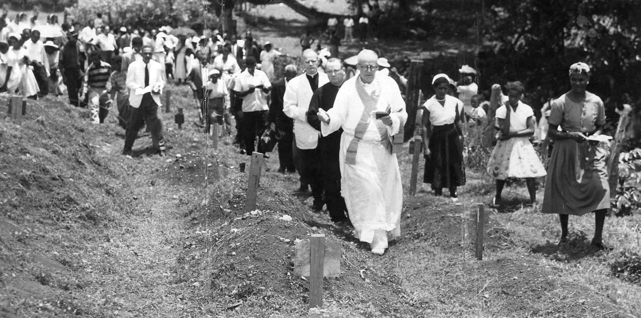
Rev Rt Charles Eberle, SJ; Rev Fr Anthony Feeherry, CP and Rev Fr William Whelan CP administering blessings at the memorial service for the unidentified
According to Gary Nieta — there were indeed more gruesome photographs taken of the crash. Those photos have not been seen publically since.

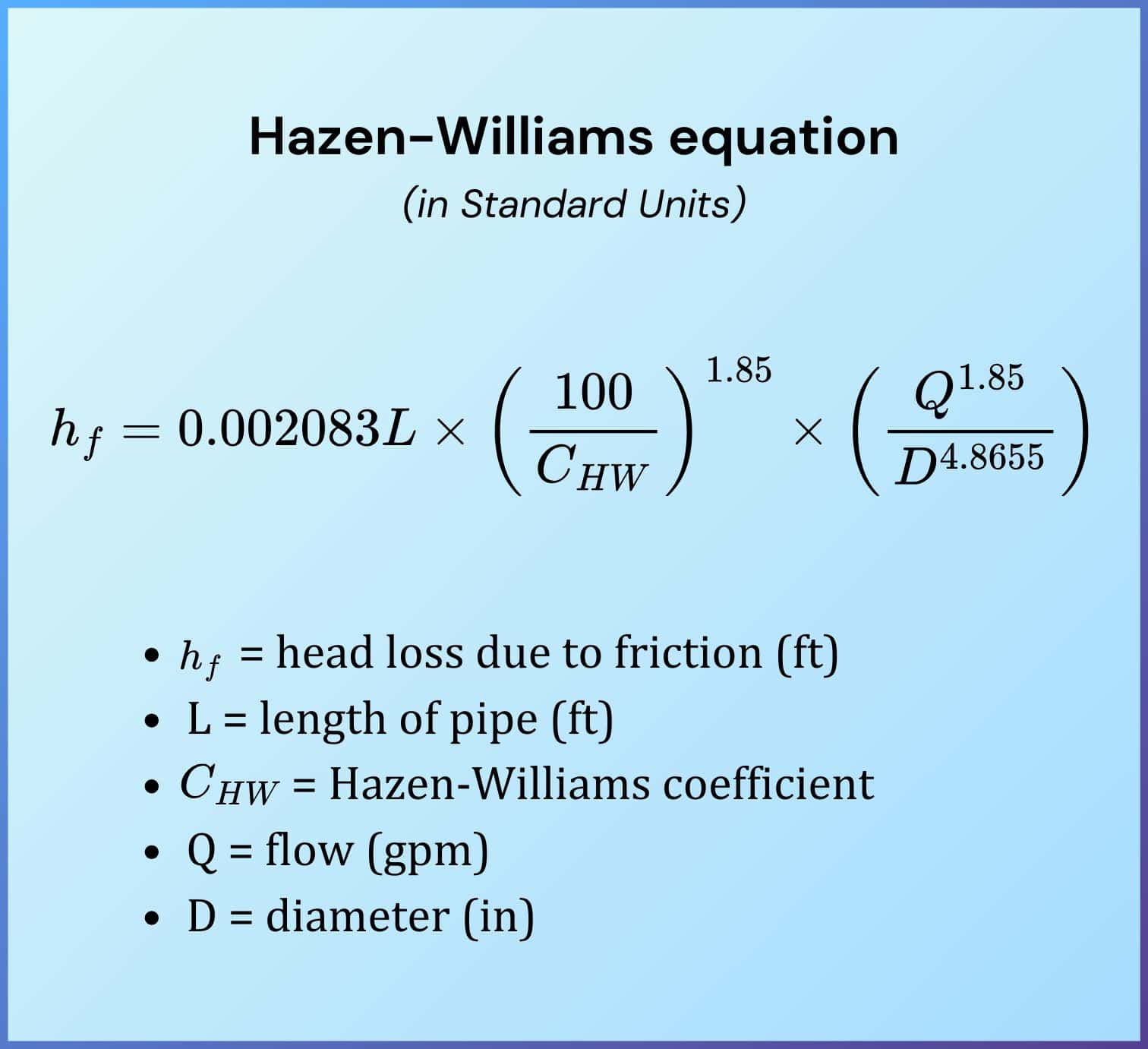
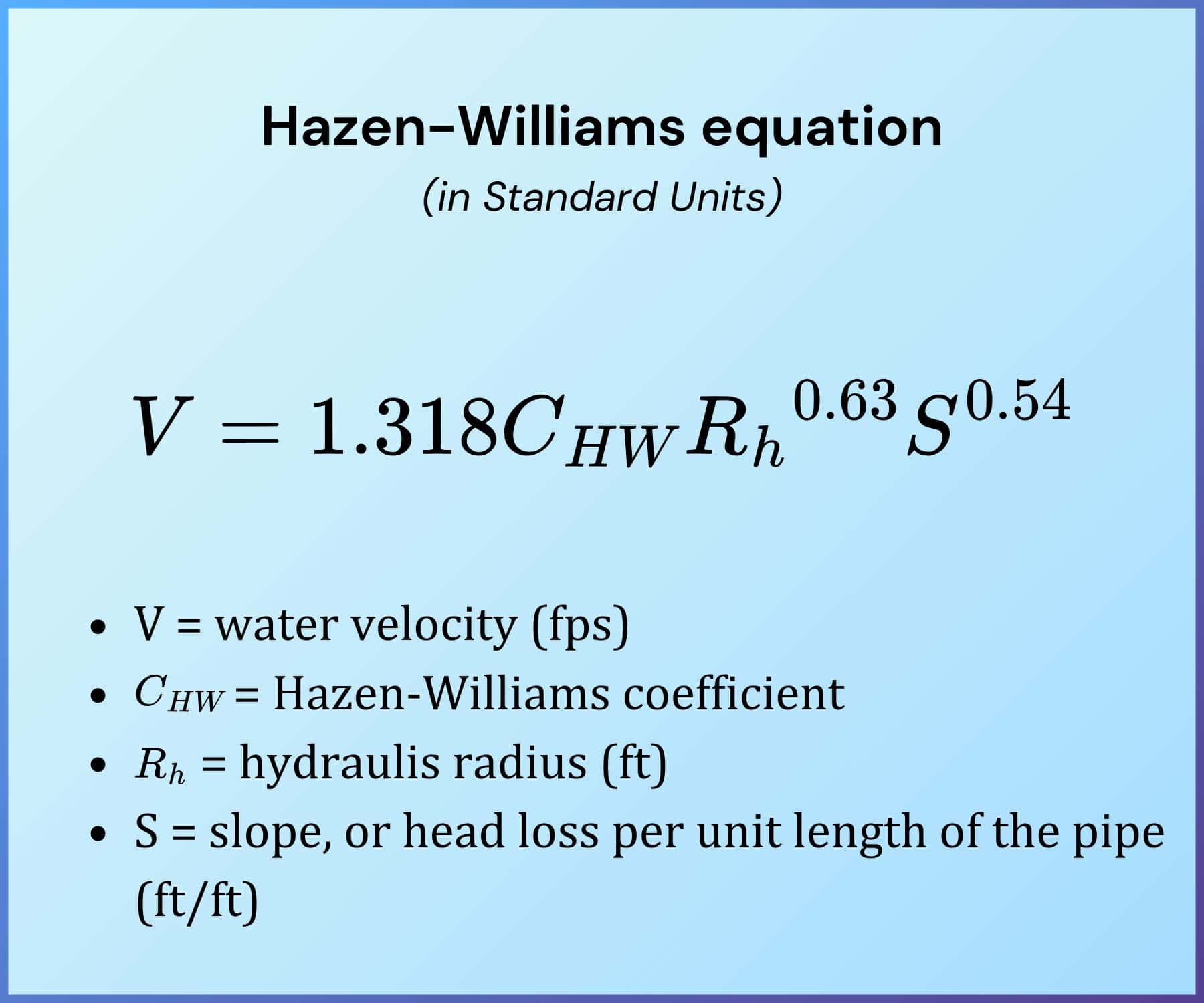
– the most popular pipe flow equation.
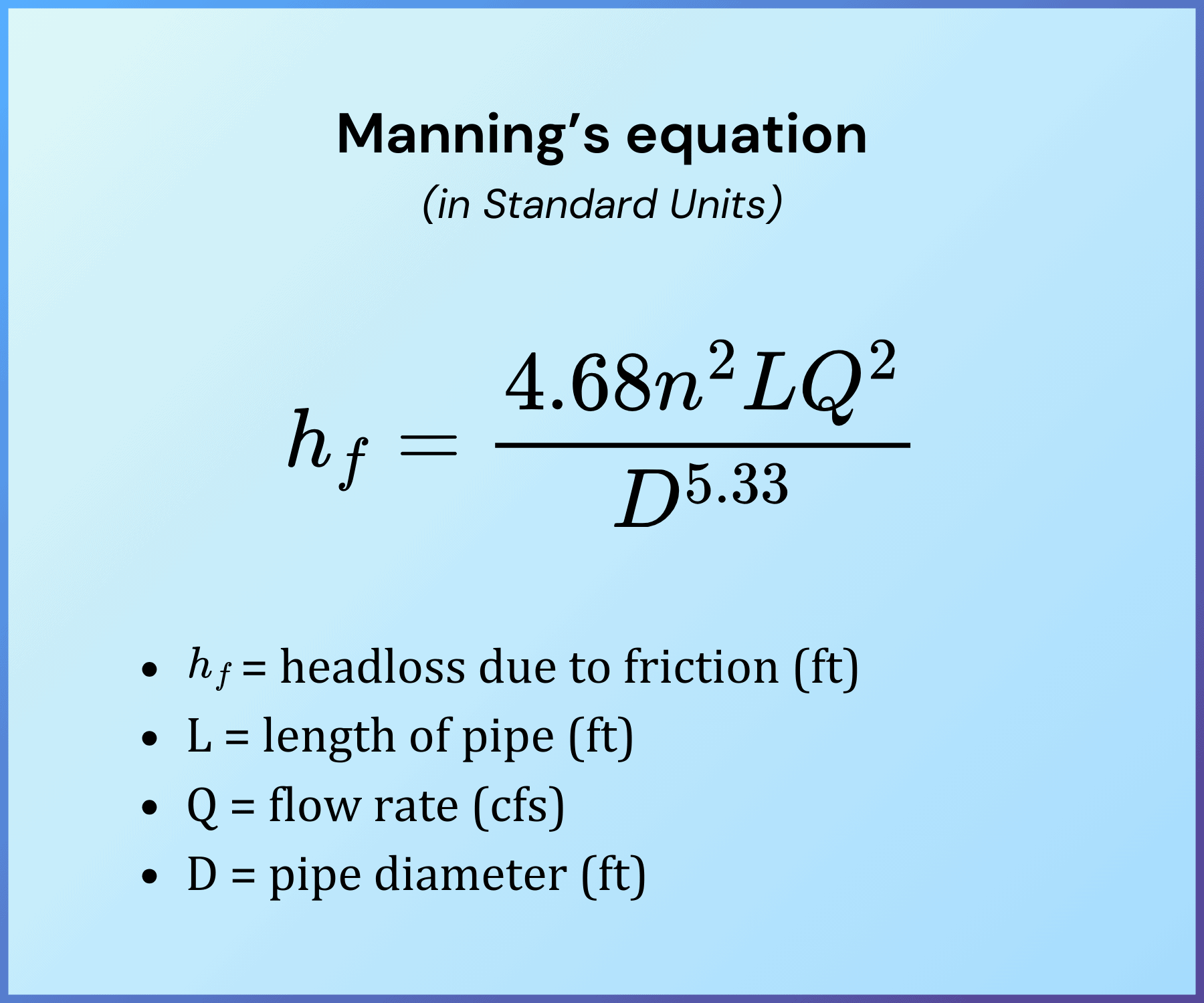
– more applicable to laminar flow and to fluids other than water.
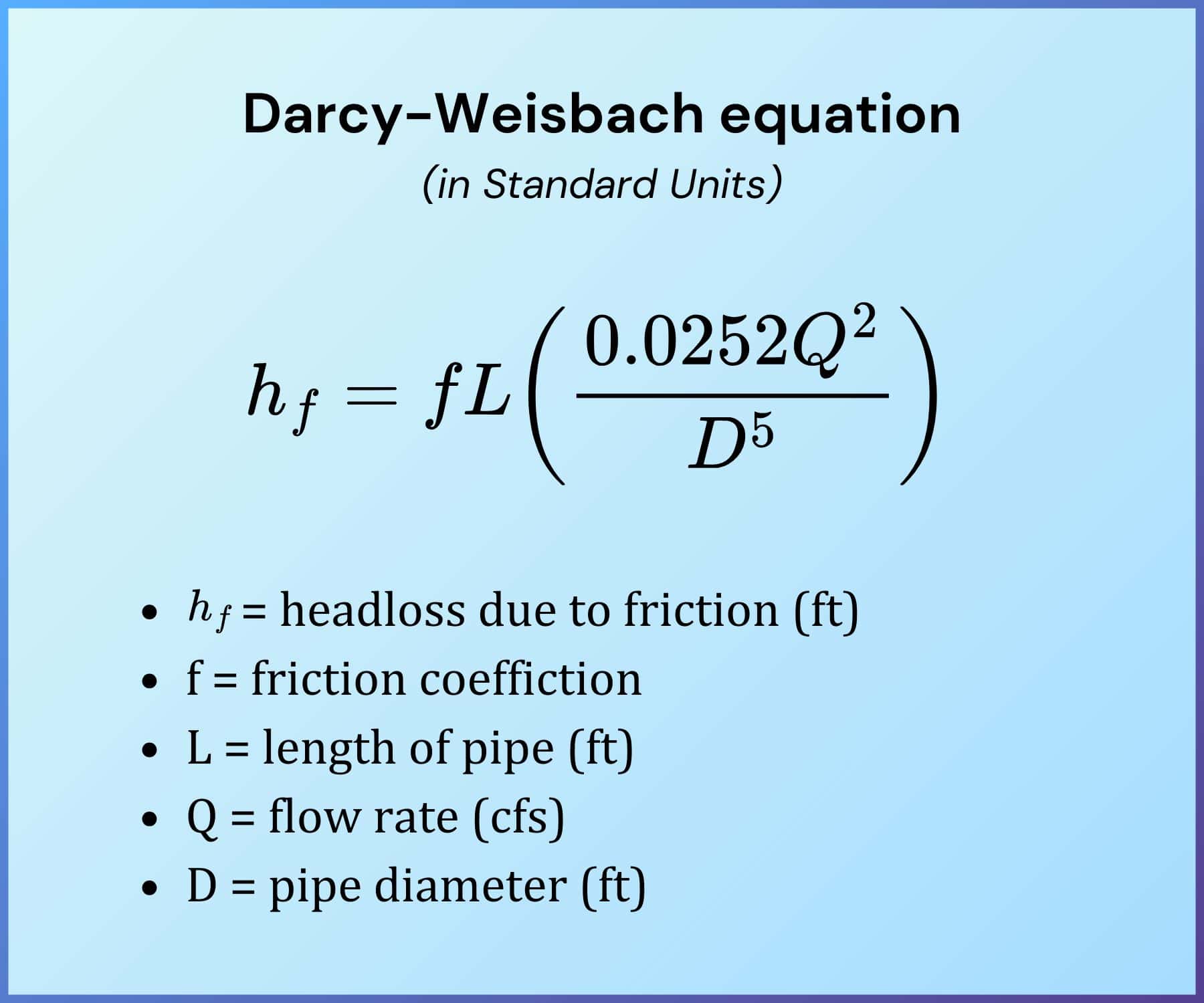
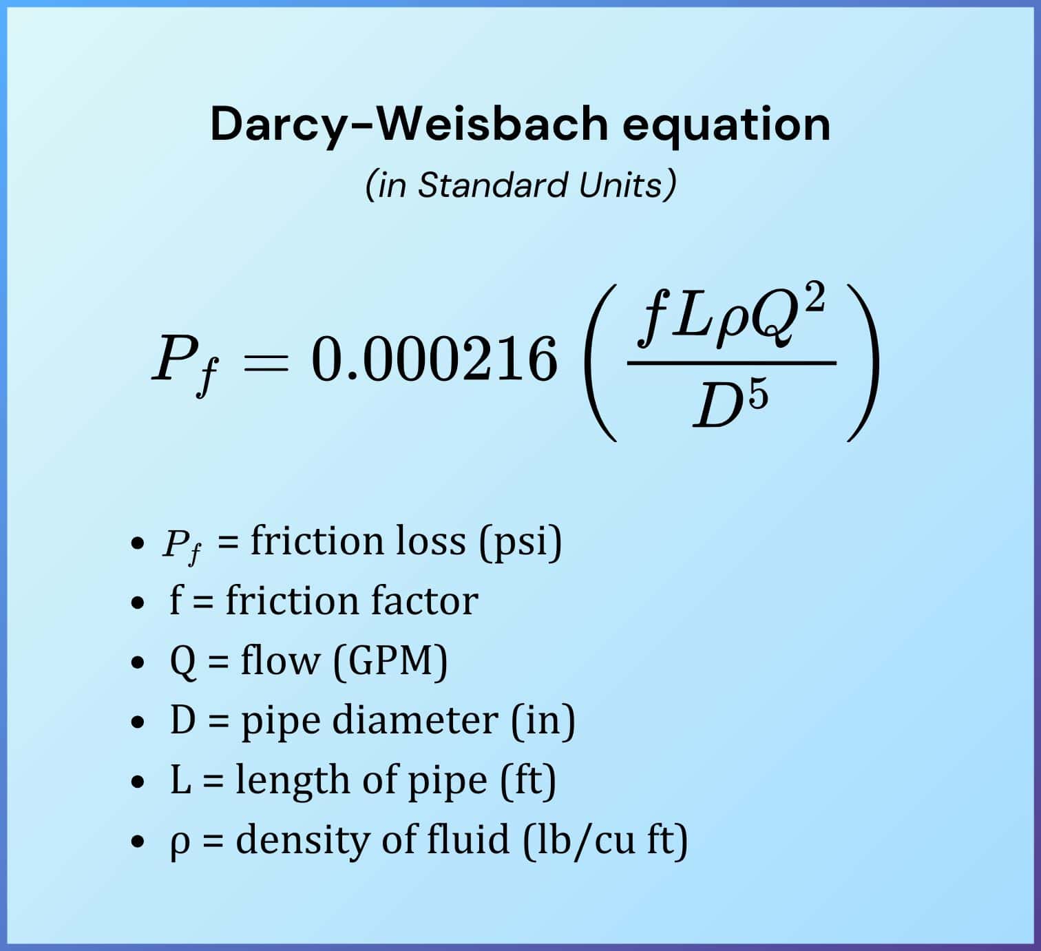
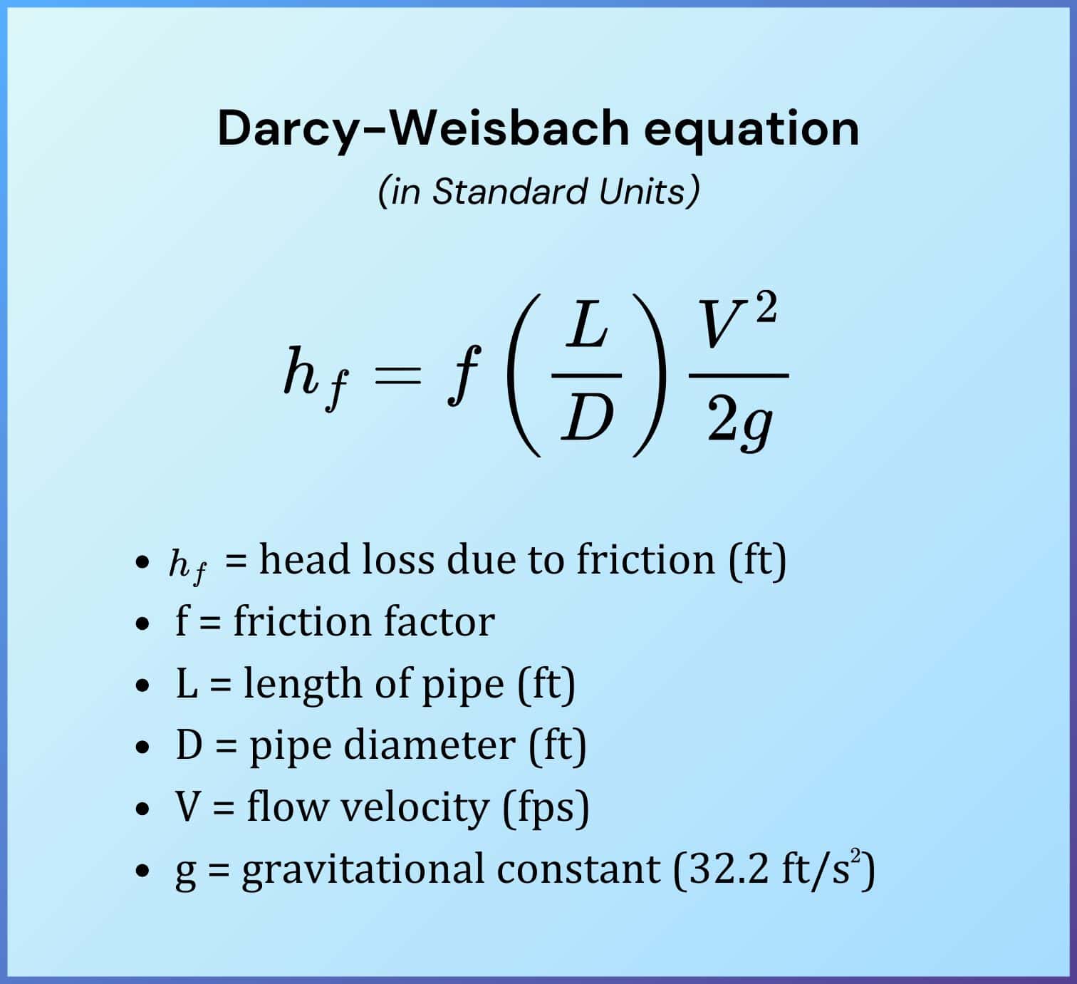
– used for pipelines with full flow meaning pressurized flow.
– used more for pipes greater than 2″ in diameter.
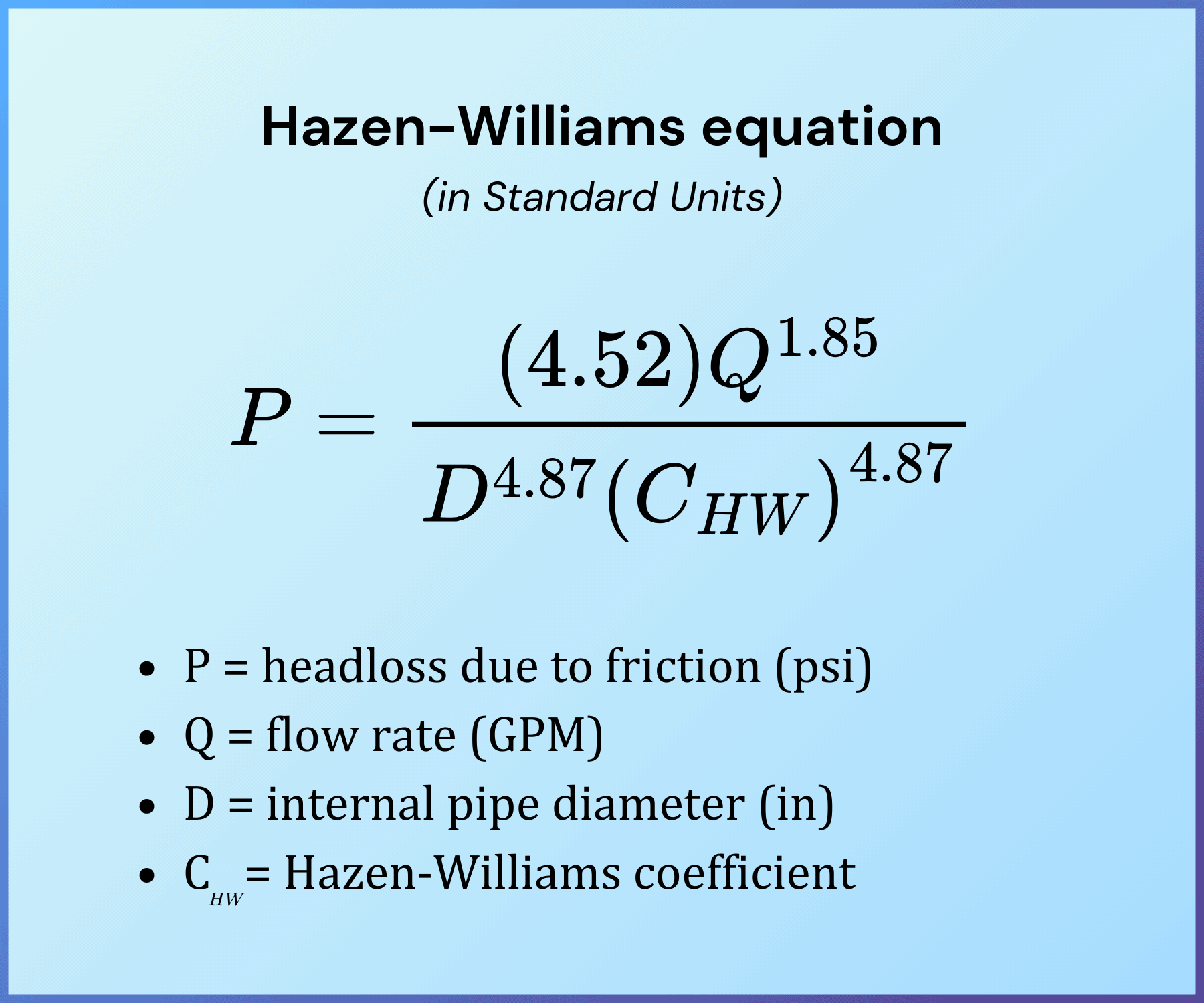
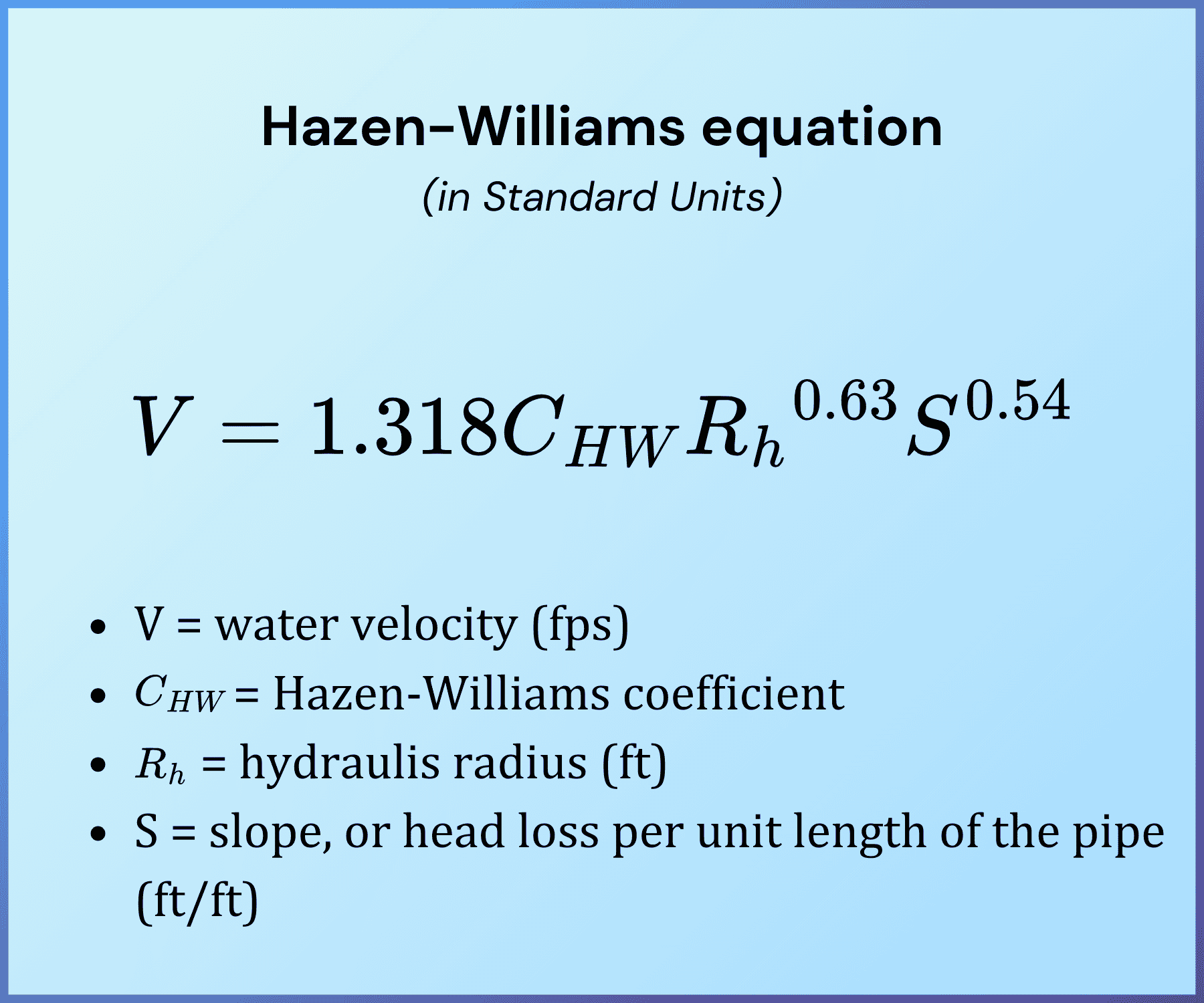
– more applicable to laminar flow and to fluids other than water
1. Collect information on performance
2. Identify existing and forecast future system performance levels
3. Identify solutions
In other words… focus on meeting the existing and forcasted travel demand
| Stage | Description of Activity |
|---|---|
| Planning | State DOTs, MPOs, & local gov’ts identify transportion needs; financial constraints need to be considered |
| Project Development | Transportation project is more clearly defined |
| Design | Design teams makes detailes PS&Es |
| Right-of-Way | Additional land needed for project is purchased |
| Construction | State or local gov’t selects contractor, he/she then builds the project |
◼ State
◼ Regional (>50,000 pop.)
◼ Local
1. Trip generation
2. Trip distribution
3. Mode split
4. Trip assignment
exmpl scenario…
Trip generation: decision to travel for a specific purpose.
— “We need somewhere to go eat lunch, Chris!”
Trip distribution: choice of destination
— “Let’s go to Wendy’s; I hear they have a 4 for 4”
Mode choice: choice of travel mode
— “There’s 3 of us, let’s travel by car”
Network assignment: choice of route or path
— “My Google Maps says there’s a Wendy’s on 441. We can get there in 9 minutes”
3 factors that influence trip productions & attraction
◼Density of land use affects production & attraction (Number of dwellings, employees, etc. per unit of land); Higher density usually = more trips
◼ Social and socioeconomic characters of users
influence production (Average family income, Education, Car ownership)
◼ Location (Traffic congestion, Environmental conditions)
Forecast # of trips that produced or attracted by each
area for a “typical” day,
Mon – Fri is usually focus only primarily
◼ Objective of a trip generation model is to forecast number of person-trios that shall begin from or end in each travel-analysis zone within the region for a typical day of said target year
◼ (HB) Home Based Trip – a trip where the home of trip-maker is either the origin or the destination
◼ (NHB) Non-Home Based Trip – a trip where the home is neither end of the trip
◼ Utility functions – what value does each user put on being able to travel (e.g. Utility of getting groceries is higher than going to the movies)
◼ Journey – this is a a one-way movement from a point of origin to a point of destinations
◼ Pi = f(z1, z2, z3, …), trip production for zone I,
◼ Ai = f(y1, y2, y3, …), trip attraction for zone I,
z factors include: (income, household structure, family size, car ownership, value of land, residential density)
y factors include: (industrial, commercial and other services, zonal employment, recreational resources)
◼ Trip Production – defined as a the home end of an HB trip, or as the origin of a NHB trip
◼ Trip Attraction – defined of the non-home-end of an HB trip or the destination of an NHB trip
◼ Trip Generation – often defined as the total number of trips generated by households in a zone be they HB or NHB
exmpl form:
Tj = b0 +b1z1j + b2z2j + … bnznj
◼ Tj is number of vehicle-based trips in a specified time period by household j
◼ Znj is characteristic n (e.g. income, employment, no. of members) of household j
◼ bn is a coefficient estimated from traveler survey data corresponding to characterstic n
T_{ij}=\frac{P_{i}(A_{j}\times F_{ij})}{\sum A_{j} \times F_{ij}}Tij = Trips from zone i to zone j
Pi = Trip production in zone i
Aj = Trip attraction in zone j
Fij = Effect of travel time & dinstance in zone i and zone j
P_{ij}=\frac{e^{\text{transit utility}_{ij}}}{e^{\text{transit utility}_{ij}}+e^{\text{auto utility}_{ij}}}Pij = Probaility of using transit for a trip between Zone i to Zone j
Transity utility ij = f (transit level of service ij, income ij)
Auto utility ij = f (highway level of service ij, income ij)
\begin{aligned}T_{i}&=F_{i}t_{i} \\ \\F_{i}&=\frac{f(P^{d}_{i},I^{d}_{i},C^{d}_{i})}{f(P^{c}_{i},I^{c}_{i},C^{c}_{i})}\end{aligned}Pij = Probaility of using transit for a trip between Zone i to Zone j
Transity utility ij = f (transit level of service ij, income ij)
Auto utility ij = f (highway level of service ij, income ij)
social